An RLC low pass filter

In what follows different ways to characterise the properties of an LTI system introduced will be reviewerd throught the example of a second-order analog low-pass filter of the type we see a lot.

We draw the circuit using schemdraw and matplotlib packages.

import schemdraw
import schemdraw.elements as elm

import matplotlib

%matplotlib inline
%config InlineBackend.figure_format = 'svg'

d = schemdraw.Drawing(fontsize=12)
d += (A1 := elm.Dot())
d += (L := elm.Inductor2().label('L'))
d += (C := elm.Capacitor().down().label('C', loc='bottom'))
d += (w1 := elm.Line().left().tox(A1.start))
d += (A2 := elm.Dot())
d += (w2 := elm.Line().right().at(C.start))
d += (R := elm.Resistor().down().label('R'))
d += (w4 := elm.Line().right().at(R.start))
d += (B1 := elm.Dot())
d += (w3 := elm.Line().right().at(C.end))
d += (w4 := elm.Line().right())
d += (B2 := elm.Dot())
d += (oc_out := elm.Gap().endpoints(B1.start, B2.end).label(['+', r'$y(t)$', '-']))
d += (oc_in := elm.Gap().endpoints(A1.start, A2.end).label(['+', r'$x(t)$', '-']))

d.draw()

---------------------------------------------------------------------------
ModuleNotFoundError                       Traceback (most recent call last)
/tmp/ipykernel_61072/788269032.py in <module>
----> 1 import schemdraw
      2 import schemdraw.elements as elm
      3 
      4 import matplotlib
      5 

ModuleNotFoundError: No module named 'schemdraw'

No energy is stored in the capacitor and inductor for \(t<0\). It is furthermore assumed that the input voltage \(x(t) = 0\) for \(t<0\). Hence \(y(t) = 0\) and \(\frac{d y(t)}{dt} = 0\) for \(t<0\). Let \(L = 0.05\), \(R = 2\), \(C = 0.040\) are used for the elements of the electrical network.

Differential Equation

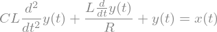
The differential equation describing the input/output relation of the electrical network is derived by applying Kirchhoff’s circuit laws to the network. This results in the following ODE

\begin{equation} C L \frac{d^2 y(t)}{dt^2} + \dfrac{L}{R} \frac{d y(t)}{dt} + y(t) = x(t) \end{equation}

This ODE is defined in SymPy

import sympy as sym
sym.init_printing()

t, L, R, C = sym.symbols('t L R C', real=True)
x = sym.Function('x')(t)
y = sym.Function('y')(t)

ode = sym.Eq(L*C*y.diff(t, 2) + (L/R)*y.diff(t) + y, x)
ode

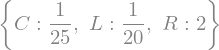
The normalized values of the network elements are stored in a dictionary for later substitution

RLC = {R: 2, L: sym.Rational('.05'), C: sym.Rational('.040')}
RLC

Impulse Response

The passive electrical network and the ODE describing its input/output relation can be interpreted as an LTI system. Hence, the system can be characterized by its impulse response \(h(t)\) which is defined as the output of the system for a Dirac Delta impulse \(x(t) = \delta(t)\) at the input. For the given system, the impulse response is calculated by explicit solution of the ODE

solution_h = sym.dsolve(
    ode.subs(x, sym.DiracDelta(t)).subs(y, sym.Function('h')(t)))
solution_h

The integration constants \(C_1\) and \(C_2\) have to be determined from the initial conditions \(y(t) = 0\) and \(\frac{d y(t)}{dt} = 0\) for \(t<0\).

integration_constants = sym.solve((solution_h.rhs.limit(
    t, 0, '-'), solution_h.rhs.diff(t).limit(t, 0, '-')), ['C1', 'C2'])
integration_constants

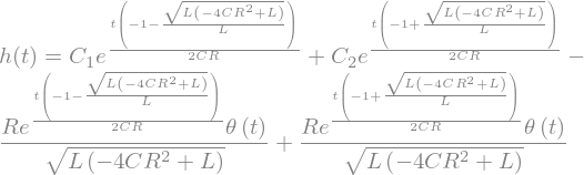
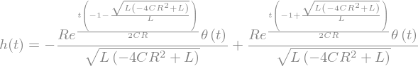
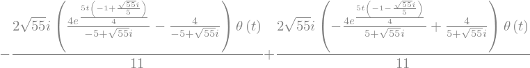
Substitution of the values for the integration constants \(C_1\) and \(C_2\) into the result from above yields the impulse response of the low-pass

h = solution_h.subs(integration_constants)
h

The impulse response is plotted for the values of \(R\), \(L\) and \(C\) given above

sym.plot(h.rhs.subs(RLC), (t, -.1, 1), ylabel=r'h(t)');

Step Response

The step response is derived by integrating over the impulse response \(h(t)\). It is the reponse of the system when a unit source is connected to the input terminal at time \(t=0\). For ease of illustration this is performed for the specific values of the elements given above

tau = sym.symbols('tau', real=True)

he = sym.integrate(h.rhs.subs(RLC).subs(t, tau), (tau, 0, t))
he

Let’s plot the step response

sym.plot(he, (t, -.1, 5), ylabel=r'$h_\epsilon(t)$');

---------------------------------------------------------------------------
NameError                                 Traceback (most recent call last)
/tmp/ipykernel_25512/1692611031.py in <module>
----> 1 sym.plot(he, (t, -.1, 5), ylabel=r'$h_\epsilon(t)$');

NameError: name 'he' is not defined

Transfer Function

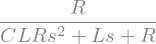
For an exponential input signal \(x(t) = e^{s t}\), the transfer function \(H(s)\) represents the complex weight of the exponential output signal \(y(t) = H(s) \cdot e^{s t}\). The transfer function is derived by introducing \(x(t)\) and \(y(t)\) into the ODE and solving for \(H(s)\)

s = sym.symbols('s')
H = sym.Function('H')(s)

H, = sym.solve(ode.subs(x, sym.exp(s*t)).subs(y, H*sym.exp(s*t)).doit(), H)
H

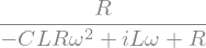
The transfer characteristic of an LTI system for harmonic exponential signals \(e^{j \omega t} = \cos(\omega t) + j \sin(\omega t)\) is of special interest for the analysis of electrical circuits. It can be derived from \(H(s)\) by substituting the complex frequency \(s\) by \(s = j \omega\). The resulting transfer function \(H(j \omega)\) provides the attenuation/amplification and phase the system adds to an harmonic input signal.

w = sym.symbols('omega', real=True)

Hjw = H.subs(s, sym.I * w)
Hjw

The magnitude of the transfer function \(|H(j \omega)|\) and its phase are plotted for illustration for values of the elements given above.

We use the control package to plot the log-log graph of the mantide and the phase of \(H(j\omega)\).

import control
import numpy

RLC = {R: 2, L: sym.Rational('.05'), C: sym.Rational('.04')}

G = control.tf(1, [float((C*L).subs(RLC).evalf()), float((L/R).subs(RLC).evalf()), 1])
omega = numpy.logspace(-2, 2, 1000)

control.bode(G, omega);