Transformers

Transformers are essential parts of most power systems. Their role is to convert electrical energy at one voltage to some other voltage. Transmission lines are typically operated at voltages that are substantially higher than either the generation or utilisation voltage, for at least two reasons.

• Because power is voltage multiplied by current, and because transmission line losses are proportional to the square of current, higher voltages generally produce lower transmission line losses.

• Transmission line capacity to carry power is roughly proportional to the square of voltage, so to make intensive use of transmission line right-of-way, that is, to enable transmission lines to carry high power levels, high transmission voltages are required. This is true for underground cables as well as for above the ground transmission lines.

For these reasons, a transformer is usually situated right at the output of each generating unit to transform the power from generation voltage, which is usually between 10 and 30 kV, and transmission voltage which is in the high or extra high voltage range, typically between 138 and 765 kV. At substations that connect transmission lines to distribution circuits the power is stepped down in voltage. Distribution circuits generally operate in the range of 6–35 kV. (However, there are still lower voltage distribution primaries and some higher voltage circuits might be classified as distribution.) Then, before electric power is connected to customer loads, there is yet another transformer to transform it from the distribution primary voltage to the customer at a voltage that is typically on the order of 240 V. In the United States that last transformer is center tapped to give the familiar 120 V, RMS, single-phase voltage used for most appliances.

Single-phase Transformers

Many transformers used in electric power systems are built as three-phase transformers. However, as seen earlier, three-phase systems can be viewed as three single-phased subsystems. We start by considering such single-phase units.

Ideal Trasnformers

A multiple winding ideal transformer is given below.

Fig. 102 A general multi-port transformer.

\[ \dfrac{v_1(t)}{n_1}=\dfrac{v_2(t)}{n_2}=\dfrac{v_3(t)}{n_3} \]

\[ n_1 i_1(t)+n_2i_2(t) +n_3 i_3(t)=0 \]

1. A transformer turns ratio between the primary and output port is often chosen so that the desired voltages appear at the proper terminals. For example, to convert 8 kV distribution voltage to the 120/240 V level suitable for residential or commercial single-phase service, one would use a transformer with a turns ratio of \(\frac{8000}{240} = 33\frac{1}{3}\). To split the low voltage in half, a center tap on the low voltage winding would be used.

2. An ideal transformer does not consume, produce or store energy. From the equations above, the sum of power flows into an ideal transformer (with multiple output windings) is identically zero: \(\sum_{i} p_i = 0\)

3. One can reflect elements through the windings of a transformer to construct equivalent circuits. The reflection of a voltage source, a current source, and an impedance through a transformer are presented below.

Note

In writing the relationship between the currents and the voltages of different ports of a transformer we can use the sinusoidal-steady state (phasor notation) representation of the currents and voltages. In other words, for the example above:

\[ \dfrac{\mathbf{V}_1}{n_1}=\dfrac{\mathbf{V}_2}{n_2}=\dfrac{\mathbf{V}_3}{n_3} \]

\[ n_1 \mathbf{I}_1+n_2\mathbf{I}_2 +n_3 \mathbf{I}_3=0 \]

where the bold variables are the phasors of the corresponding circuit variable.

Non-Idealities in Transformers

Real transformers behaviour differs from the ideal case due to two major factors. One is related to the transformer cores themselves, and the second is due to the resistance and leakage reactance of the transformer windings.

Transformers are wound on magnetic circuits (cores) made of thin sheets, called laminations, of steel. The core material draws some reactive power and has losses from hysteresis and eddy currents. The reactive power and loss might be approximated by shunt (parallel) reactive and resistive elements.

If real and reactive power drawn by the core are \(P_c\) and \(Q_c\), respectively, the resistance and reactance elements that describe transformer behaviour are

\[ R_\phi \approx \dfrac{V_1^2}{P_c},\quad X_\phi \approx \dfrac{V_1^2}{Q_c} \]

where \(V_1\) is the magnitude of the voltage at the primary. Assuming that the transformer has \(n_1\) turns in the winding connected to the voltage of magnitude \(V_1\) and frequency \(\omega\), and that the core itself has an area \(A_c\), then the flux density in the core is

\[ B_c \approx \dfrac{V_1}{\omega n_1 A_c}. \]

It is possible to use tabulated data on core materials in conjunction with the flux density \(B_c\) and frequency \(\omega\) to deduce a watts per kilogram and a VARs per kilogram number for a given core material. The values of \(P_c\) and \(Q_c\) are then calculated by using those two numbers and multiplying by the mass of the core. It is important to realise here that the behaviour of magnetic iron is nonlinear with respect to flux density, so these resistive and reactive core elements are only approximations to actual transformer behaviour, and their values will be functions of operating point. Core loss is a very important element of transformer behaviour since power transformers in utility systems are virtually always energised, so that “no-load” loss in power transformers is relatively expensive.

The windings in the power transformer, of course, have resistance. They also make magnetic flux, not all of which is mutually coupled.

Note

The flux in the core is all mutually coupled, but there will be some leakage flux in the air around the core, and this is what gives rise to the leakage flux elements.

The circuit model of a nonideal transformer with is given below:

Fig. 103 A nonideal transformer model.

Reflecting the elements from the secondary yields:

Fig. 104 A nonideal transformer model with all elements on the primary side.

where

\[ R = R_1 + \left ( \dfrac{n_1}{n_2} \right )^2 R_2, \quad X = X_1 + \left ( \dfrac{n_1}{n_2} \right )^2 X_2 \]

and \(n_1/n_2\) is the turn ratio of the primary to the secondary windings.

Typically, the core elements of the power transformer are fairly large, so they have little effect on the behaviour of the power system, although the core loss element is economically important. Also, the series resistance tends to be quite small, so in system studies it is often found that only the series leakage reactance need be represented.

Autotransformers

A special transformer connection is shown in Fig. 105, called an autotransformer: two windings on the same core are connected in series. If the two windings have \(n_1\) and \(n_2\) turns, respectively, the voltages and currents are

Fig. 105 An autotransformer

An equivalent representation of an autoransformer is given in the right-most figure above.

From transformer equations we have:

\[ \dfrac{v_a-v_b}{n_1} = \dfrac{v_b-v_c}{n_2} \]

It is common in applications for ground the \(c\) terminal. Thus,

\[ v_a = \dfrac{n_1+n_2}{n_2}v_b \]

Similarly, for the currents we obtain

\[ i_a = \dfrac{n_2}{n_1+n_2}i_b \]

where \(i_b\) is the current exiting the middle tap.

Hence, an autotransformer with grounded \(c\) can be seen as a transformer with turn ratio of \(N = 1 + \dfrac{n_1}{n_2}\). The rating (colloquial for the total power transferred through the transformer), denoted by \(VA\) is:

\[ VA = v_a i_a = v_b i_b \]

The motivation for winding a transformer this way is that it uses less material than a two winding transformer, for which the total winding rating must be \(2VA\) because there are two windings, both carrying the same product of volts and amperes. The ratings of windings of an autotransformer are

\[ VA_1 = (v_a -v_b) i_a = v_a i_a \left (1-\dfrac{1}{N} \right ) \]

\[ VA_2 = v_b (i_a-i_b) = v_b i_b \left (1-\dfrac{1}{N} \right ) \]

The sum of the two winding ratings is \(2 VA \left (1-\dfrac{1}{N} \right )\).

If the voltage ratio is not large, there can be appreciable savings in material. Autotransformers are often used for connection between very high and extra high voltage circuits where the ratio of voltages is not very large, such as connecting 138 and 345 kV circuits. They are also used in transformer isolated switched power converters.

Three-phase Transformers

Polyphase transformers can be implemented as three single-phase transformers or as three sets of winding on a suitable core. A set of windings, each constituting a single-phase transformer, would be wound around each leg of this three-legged core.

A three-phase transformer operates as three single-phase transformers. The complication is that there are a number of ways of winding them and a number of ways of interconnecting them. On either side of a transformer connection (i.e. the high-voltage and low-voltage sides), it is possible to connect transformer windings either line to neutral (wye) or line to line (delta). Thus we may speak of transformer connections being wye–wye, delta–delta, wye–delta, or delta–wye. Connection of transformers in either wye–wye or delta–delta is reasonably easy to understand. Each of the line–neutral (in the case of wye–wye) or line–line (in the case of delta–delta) voltages is transformed by one of the three transformers. On the other hand, the interconnections of wye–delta or delta–wye transformers are a little more complex. Fig. 106 depicts a delta–wye connection. In that picture, winding elements that appear parallel are wound on the same core segment, and so constitute a single-phase transformer.

One might ask why bother with delta connections in the first place. As it turns out, transformer cores are nonlinear and draw harmonic currents. Third harmonic currents are in phase with each other, leading to currents flowing into the neutral connection in a wye, but that simply circulate around a delta. Thus in order to keep the core happy, most transformer connections include a delta on one side or the other. On the other hand, in order to load phase to ground, one needs to have a wye connection. Thus many situations involve a delta/wye, where the wye is on the side to be loaded.

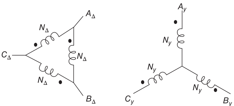
Fig. 106 A a delta–wye transformer

Assume that \(N_{\Delta}\) and \(N_Y\) are numbers of turns. If the individual transformers are considered to be ideal, then:

\[\begin{split} \begin{aligned} v_{aY} & = \dfrac{N_Y}{N_{\Delta}} (v_{a\Delta} - v_{b\Delta}),\qquad i_{a\Delta} = \dfrac{N_Y}{N_{\Delta}} (i_{aY} - i_{cY})\\ v_{bY} & = \dfrac{N_Y}{N_{\Delta}} (v_{b\Delta} - v_{c\Delta}),\qquad i_{b\Delta} = \dfrac{N_Y}{N_{\Delta}} (i_{bY} - i_{aY})\\ v_{cY} & = \dfrac{N_Y}{N_{\Delta}} (v_{c\Delta} - v_{a\Delta}),\qquad i_{c\Delta} = \dfrac{N_Y}{N_{\Delta}} (i_{cY} - i_{bY}) \end{aligned} \end{split}\]

where each of the voltages are line–neutral and the currents are in the lines at the transformer terminals. Consider the case where a delta–wye transformer is connected to a balanced three-phase voltage source:

\[\begin{split} \begin{aligned} v_{a\Delta} &= \Re\left \{\mathbf{V} \mathrm{e}^{\jmath \omega t} \right \}, \\ v_{b\Delta} &= \Re\left \{\mathbf{V} \mathrm{e}^{\jmath (\omega t-\frac{2\pi}{3})}\right \}\\ v_{c\Delta} &= \Re\left \{\mathbf{V} \mathrm{e}^{\jmath (\omega t + \frac{2\pi}{3})}\right \} \end{aligned} \end{split}\]

Then, the complex amplitudes on the wye side are

\[\begin{split} \begin{aligned} \mathbf{V}_{aY} &= \dfrac{N_Y}{N_{\Delta}} \mathbf{V} \left (1- \mathrm{e}^{-\jmath \frac{2\pi}{3}} \right ) = \sqrt{3} \dfrac{N_Y}{N_{\Delta}}\mathbf{V} \mathrm{e}^{\frac{\jmath\pi}{6}}, \\ \mathbf{V}_{bY} &= \dfrac{N_Y}{N_{\Delta}}\mathbf{V} \left ( \mathrm{e}^{-\jmath \frac{2\pi}{3}} - \mathrm{e}^{\jmath \frac{2\pi}{3}}\right )= \sqrt{3} \dfrac{N_Y}{N_{\Delta}}\mathbf{V}\mathrm{e}^{ \frac{-\jmath\pi}{2}}\\ \mathbf{V}_{cY} &= \dfrac{N_Y}{N_{\Delta}} \mathbf{V} \left ( \mathrm{e}^{\jmath \frac{2\pi}{3}} -1 \right )= \sqrt{3} \dfrac{N_Y}{N_{\Delta}}\mathbf{V}\mathrm{e}^{\frac{\jmath 5 \pi }{6}} \end{aligned} \end{split}\]

Note

• The ratio of voltages (i.e. the ratio of either line–line or line–neutral) is different from the turns ratio by a factor of \(\sqrt{3}\).

• All wye side voltages are shifted in phase by \(30^\circ\) with respect to the delta side voltages.

Example 4

A balanced three-phase wye-connected resistor is connected to the delta side of a wye–delta transformer with a nominal voltage ratio of

\[ \dfrac{v_{\Delta}}{v_y} = N \]

as depicted below.

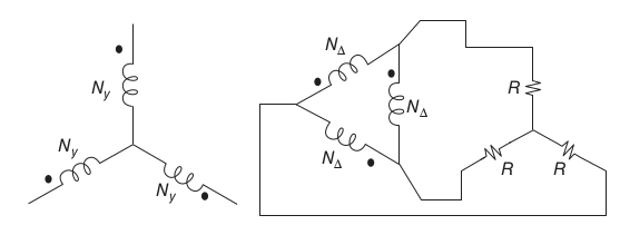
What is the impedance looking into the wye side of the transformer, assuming drive with a balanced source?

The relationship between the voltage ratio and the turns ratio is

\[ \dfrac{v_{\Delta}}{v_y} = N = \dfrac{N_{\Delta}}{\sqrt{3}N_Y}. \]

Applyintg the wye–delta equivalent transform to the load yields:

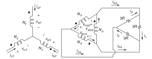
each transformer secondary winding is connected directly across one of the three resistors. Currents in the resistors are given by

\[\begin{split} \begin{aligned} i_1 &= \dfrac{v_{ab\Delta}}{3R}\\ i_2 &= \dfrac{v_{bc\Delta}}{3R}\\ i_3 &= \dfrac{v_{ca\Delta}}{3R} \end{aligned} \end{split}\]

Line currents are:

\[\begin{split} \begin{aligned} i_{a\Delta} &= i_1 - i_3= \dfrac{v_{ab\Delta} - v_{ca\Delta}}{3R} = i_{1\Delta} - i_{3\Delta}\\ i_{b\Delta} &= i_2-i_1 = \dfrac{v_{bc\Delta}-v_{ab\Delta}}{3R}= i_{2\Delta} - i_{1\Delta}\\ i_{c\Delta} &= i_3-i_2 = \dfrac{v_{ca\Delta}-v_{bc\Delta}}{3R}= i_{3\Delta} - i_{2\Delta} \end{aligned} \end{split}\]

Solving for currents in the legs of the transformer \(\Delta\), subtract, for example, the second expression from the first:

\[ 2i_{1\Delta} - i_{2\Delta} - i_{3\Delta} = \dfrac{2v_{ab\Delta} - v_{bc\Delta}- v_{ca\Delta}}{3R} \]

The system is balance, i.e.,

\[ i_{1\Delta} + i_{2\Delta} + i_{3\Delta} =0, \]

\[ v_{ab\Delta} + v_{bc\Delta} + v_{ca\Delta} = 0. \]

Hence,

\[\begin{split} \begin{aligned} i_{1\Delta} &= \dfrac{v_{ab\Delta} }{3R} \\ i_{2\Delta} &= \dfrac{v_{bc\Delta}}{3R}\\ i_{3\Delta} &= \dfrac{v_{ca\Delta}}{3R} \end{aligned} \end{split}\]

From the ideal transformer relations:

\[\begin{split} \begin{aligned} v_{ab\Delta} &= \dfrac{N_{\Delta}}{N_Y} v_{aY}, \qquad i_{aY} = \dfrac{N_{\Delta}}{N_Y} i_{1\Delta}\\ v_{bc\Delta} &= \dfrac{N_{\Delta}}{N_Y} v_{bY}, \qquad i_{bY} = \dfrac{N_{\Delta}}{N_Y} i_{2\Delta}\\ v_{ca\Delta} &= \dfrac{N_{\Delta}}{N_Y} v_{cY}, \qquad i_{cY} = \dfrac{N_{\Delta}}{N_Y} i_{3\Delta}\\ i_{aY} &= \left ( \dfrac{N_{\Delta}}{N_Y} \right )^2 \dfrac{v_{aY}}{3R}\\ i_{bY} &= \left ( \dfrac{N_{\Delta}}{N_Y} \right )^2 \dfrac{v_{bY}}{3R}\\ i_{cY} &= \left ( \dfrac{N_{\Delta}}{N_Y} \right )^2 \dfrac{v_{cY}}{3R} \end{aligned} \end{split}\]

The apparent resistance (i.e. the resistance value reflected to the wye side) at the wye terminals of the transformer is

\[ R_{eq}= 3R \left ( \dfrac{N_Y}{N_{\Delta}} \right )^2 \]

Expressed in voltage ratio \(v_Y/v_\Delta\):

\[ R_{eq}= 3R \left ( \dfrac{N}{\sqrt{3}} \right )^2 = R \left ( \dfrac{v_Y}{v_\Delta} \right )^2. \]

It is important to note that this solution took the long way around. Taken consistently (uniformly on a line–neutral or uniformly on a line–line basis), impedances transform across transformers by the square of the voltage ratio, no matter what connection is used.

Summary

We were reintroduced to transformers. We saw their ideal and nonideal models. We further investigated how they behave in three-phase interconnections.